
Influence of relative spacing (a/d) on the aerodynamic drag of a vertical cable route
Introduction
In telecommunications structures, it is often necessary to route multiple cables along a tower or mast. Due to their length and location, these cables are subject to significant wind loads. The magnitude of these loads depends, among other factors, on the cable diameter, wind velocity and the relative positioning of the cables.
When several cables are situated close to each other, significant aerodynamic interactions may occur - such as shielding or mutual flow reinforcement - which affect the total aerodynamic drag of the system.
The objective of this analysis is to quantitatively evaluate the influence of the relative positioning of cables in a bundle on the total aerodynamic drag coefficient. The focus is on a typical configuration of an overhead cable route attached to a steel mast, where the cables are routed parallel in a horizontal plane.
To enable the analysis of various geometric variants while maintaining a reasonable computation time, a two-dimensional (2D) model was adopted, in which the cross-section of the system is treated as infinitely long in the axial direction. Such an approach represents a compromise between accuracy and computational effort - it allows capturing the key aerodynamic phenomena related to the interaction of adjacent cylinders at a significantly lower time and hardware cost compared to a full 3D analysis.
The results of this study can be helpful in designing cable systems on towers and masts, especially where limiting wind loads is crucial.
Aerodynamic Analysis
As part of evaluating the wind impact on structural members, a simplified model of a system of 10 parallel cylinders with an equal diameter of d = 15 mm was developed, representing cables arranged in a single plane. The geometry was analyzed in 2D as a cross-section through the system - this enables accurate representation of aerodynamic phenomena.
The spacing between the cables was designated as a, and the basis of the analysis was the dimensionless ratio (a/d), which allows for a broader comparison of the results.

Figure 1: Schematic cross-section of the analyzed cylinder system in 2D, indicating the diameter d, spacing a and airflow direction.
Numerical Approach
The Computational Fluid Dynamics (CFD) method was applied, which involves simulating the airflow around the analyzed system by dividing the computational domain into a discrete mesh.
This allows for the representation of local changes in pressure, velocity, forces acting on the object and consequently - the determination of aerodynamic coefficients.
FloEFD software, integrated with the Solid Edge CAD system, was used to conduct the analysis. The program utilizes the k-Ɛ RNG turbulence model, which accurately represents flows with high velocity gradients - such as flow separations or wakes behind obstacles.
Wall functions were applied in the near-wall boundary zones to model velocity gradients and viscous effects close to the cable surfaces. The simulations were performed in steady-state mode, without structural dynamics analysis (no Fluid-Structure Interaction, FSI). This means that resonance phenomena and time-varying forcing forces were not taken into account. In practice - for real structures - an appropriate structural factor should be applied in accordance with PN-EN 1993-3-1; however, it was not the subject of this analysis.
Environmental Parameters
The following environmental parameters were adopted:
- Air density: 1,25 [kg/m3]
- Base pressure: 1013 [hPa]
- Ambient temperature: 20 [°C]
- Kinematic viscosity of air: 15 × 10-5 [m2/s]
- Gravity: 9,81 [m/s2]
- The analysis was conducted as a steady flow, i.e., invariant over time.
These values correspond to standard reference conditions for engineering analyses.
The analyses were performed at a preset wind velocity of 35 m/s. This value was selected based on engineering experience and available reference data and it is typical for aerodynamic calculations of this type of objects.
Determination of the Drag Coefficient
For each case (i.e., a given value of a/d), the drag force acting on the cable set was calculated, and then the average aerodynamic drag coefficient Cf was determined using the following definitions:
F– drag force acting on the cable set [N]
A – frontal surface area of the cable set [m2]
ρ – air density [kg/m3]
Computational Mesh
A computational mesh with a hexahedral structure was created for the prepared CAD model, varying in density depending on local analysis requirements. Mesh refinement was applied automatically throughout the domain - both in the areas near the cable surfaces and in their vicinity, especially behind obstacles where significant flow changes occur. Additionally, manual mesh refinements were applied in key regions close to the cables to improve the accuracy of the results.
The figures below outline the cross-sections of the computational mesh - both general views of the domain and local close-ups of areas with increased mesh density.
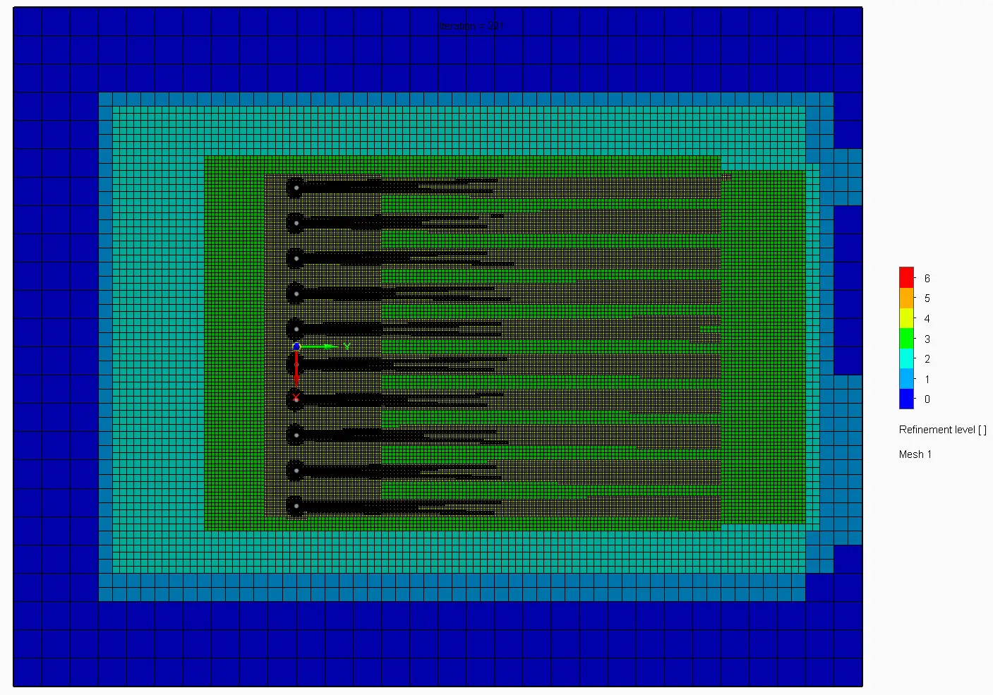
Figure 2: Base computational mesh – horizontal cross-section
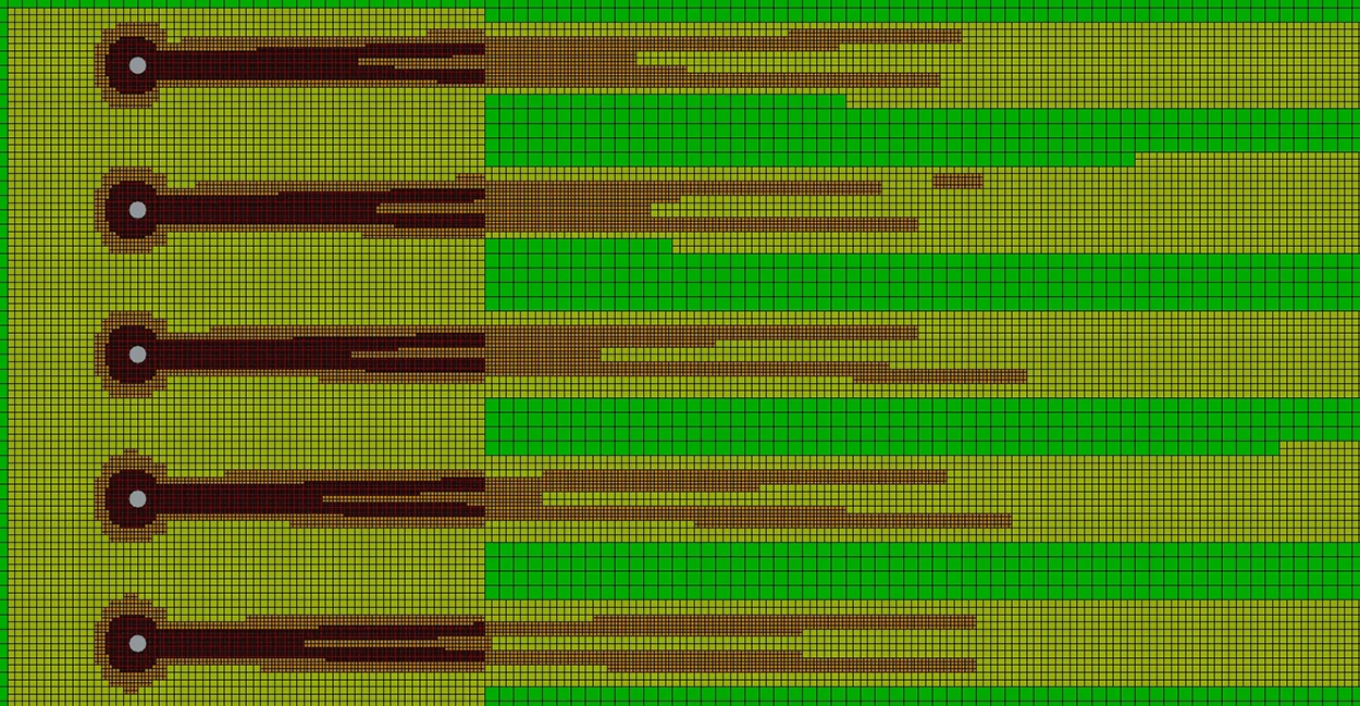
Figure 3: Base computational mesh – horizontal cross-section – detailed view
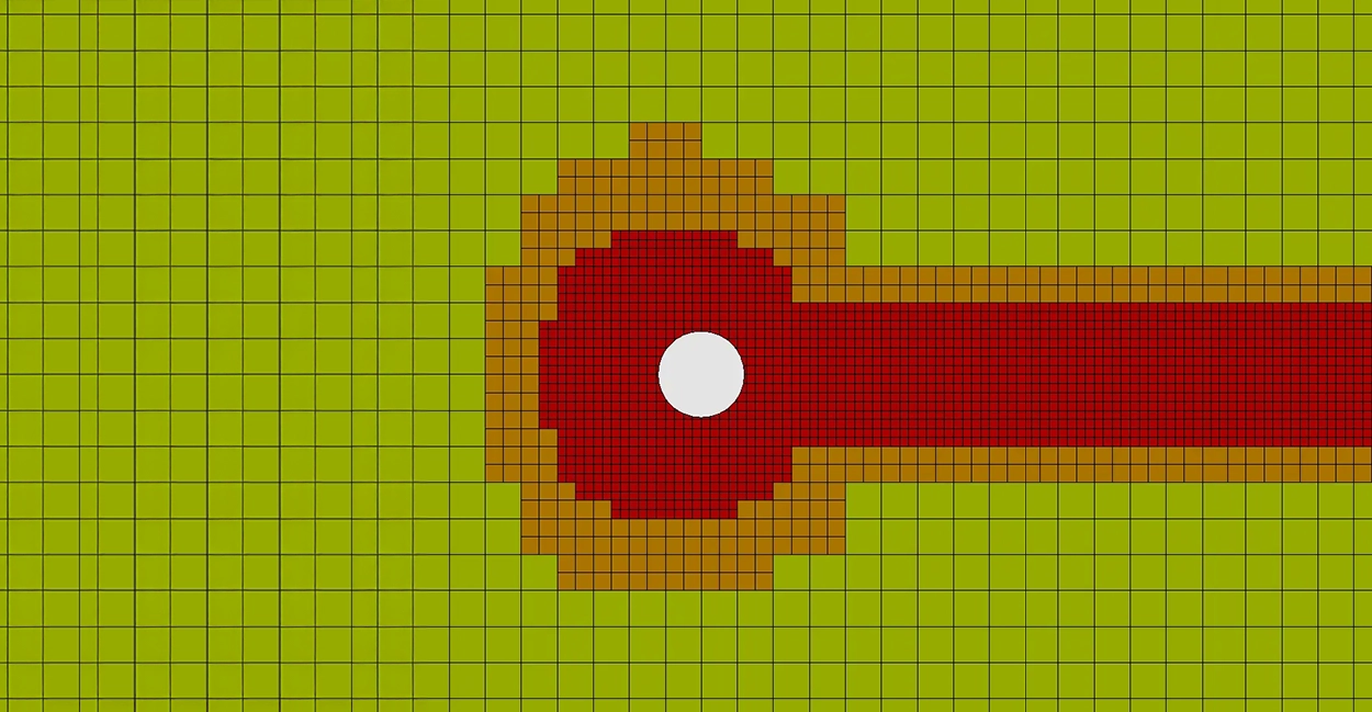
Figure 4: Base computational mesh – horizontal cross-section – view of a single cable
Presentation of Results
As part of the CFD analysis, the aerodynamic force acting on the model was determined for various values of the distance a, with a constant dimension of d = 15 mm. Based on this, the dimensionless ratio a/d and the corresponding aerodynamic coefficients Cf were calculated. These results are summarized in the table below.
| a [mm] | F [N] | a/d [-] | Cd [-] |
|---|---|---|---|
| 1.00 | 2.80 | 0.07 | 1.36 |
| 1.10 | 2.73 | 0.07 | 1.33 |
| 1.21 | 2.64 | 0.08 | 1.28 |
| 1.32 | 2.67 | 0.09 | 1.32 |
| 1.44 | 2.55 | 0.10 | 1.26 |
| 1.56 | 2.64 | 0.11 | 1.31 |
| 1.69 | 2.45 | 0.12 | 1.22 |
| 1.83 | 2.64 | 0.13 | 1.32 |
| 1.98 | 2.58 | 0.14 | 1.31 |
| 2.14 | 2.75 | 0.14 | 1.33 |
| 2.36 | 2.68 | 0.16 | 1.30 |
| 2.59 | 2.71 | 0.17 | 1.31 |
| 2.85 | 2.63 | 0.19 | 1.27 |
| 3.14 | 2.55 | 0.21 | 1.23 |
| 3.45 | 2.59 | 0.23 | 1.25 |
| 3.80 | 2.61 | 0.26 | 1.25 |
| 4.18 | 2.49 | 0.28 | 1.21 |
| 4.59 | 2.40 | 0.31 | 1.16 |
| 5.05 | 2.21 | 0.34 | 1.06 |
| 5.55 | 2.14 | 0.37 | 1.02 |
| 6.09 | 2.06 | 0.41 | 0.97 |
| 6.70 | 1.96 | 0.45 | 0.91 |
| 7.37 | 1.84 | 0.50 | 0.85 |
| 8.10 | 1.75 | 0.55 | 0.80 |
| 8.91 | 1.63 | 0.61 | 0.73 |
| 9.80 | 1.51 | 0.67 | 0.66 |
| 10.78 | 1.42 | 0.74 | 0.62 |
| 11.86 | 1.34 | 0.81 | 0.58 |
| 13.05 | 1.29 | 0.89 | 0.56 |
| 14.35 | 1.23 | 0.98 | 0.53 |
| 15.78 | 1.17 | 1.08 | 0.51 |
| 17.35 | 1.14 | 1.19 | 0.51 |
| 19.06 | 1.10 | 1.31 | 0.48 |
| 20.91 | 1.06 | 1.44 | 0.45 |
| 22.93 | 1.01 | 1.58 | 0.43 |
| 25.12 | 0.99 | 1.73 | 0.42 |
| 27.50 | 0.96 | 1.90 | 0.41 |
| 30.07 | 0.94 | 2.07 | 0.40 |
| 32.87 | 0.91 | 2.26 | 0.39 |
| 35.90 | 0.89 | 2.47 | 0.38 |
| 39.18 | 0.86 | 2.69 | 0.37 |
| 42.73 | 0.83 | 2.93 | 0.36 |
| 46.57 | 0.82 | 3.19 | 0.35 |
Table 1: Summary of CFD analysis results.
Based on the data presented in the table, a graph was prepared showing the dependence of the drag coefficient Cf on the dimensionless parameter a/d, defined as the ratio of the distance between the axes of adjacent cables to their diameter. This graph graphically illustrates the impact of changing the cable spacing on the aerodynamic characteristics of the bundle.
Using the a/d parameter allows for the generalization of the results - regardless of the specific cable diameter - which facilitates their application in various design cases. This presentation format allows for the quick identification of trends, such as the decrease or stabilization of the Cf value with increasing spacing, as well as the identification of ranges where strong aerodynamic interaction between the cables occurs.
To capture the general trend of changes in the Cf coefficient with an increase in the a/d parameter, a logarithmic trendline fitted to the calculation results was plotted on the graph. Its equation has the form: Cf = -0.252 * ln(a/d) + 0.788
The coefficient of determination is R2 = 0.954, indicating a very good fit of the model to the obtained data. The equation and the R2 value were also placed directly on the graph.

Graph 2. Dependency of the drag coefficient Cf on the a/d ratio
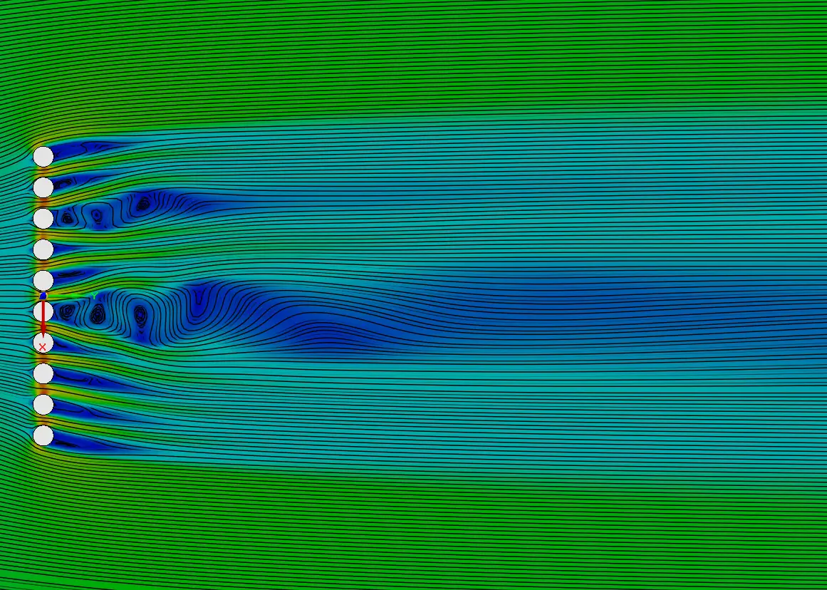
To illustrate the nature of the flow, velocity fields in the vertical plane were shown for three selected geometric cases: a/d < 1; 1 < a/d < 3; and a/d > 3. This comparison allows tracing how the velocity distribution in the space between the cables changes depending on their relative positioning.
- For the smallest distances (a/d < 1), the flow is highly disturbed, and distinct zones of decelerated flow form between the cables.
- In the intermediate range (1 < a/d < 3), a gradual stabilization of the streamlines and an increase in velocity in the inter-cable spaces are observed.
- For the largest distances (a/d > 3), the flow profiles become more symmetrical and similar to the case of a single cylinder.
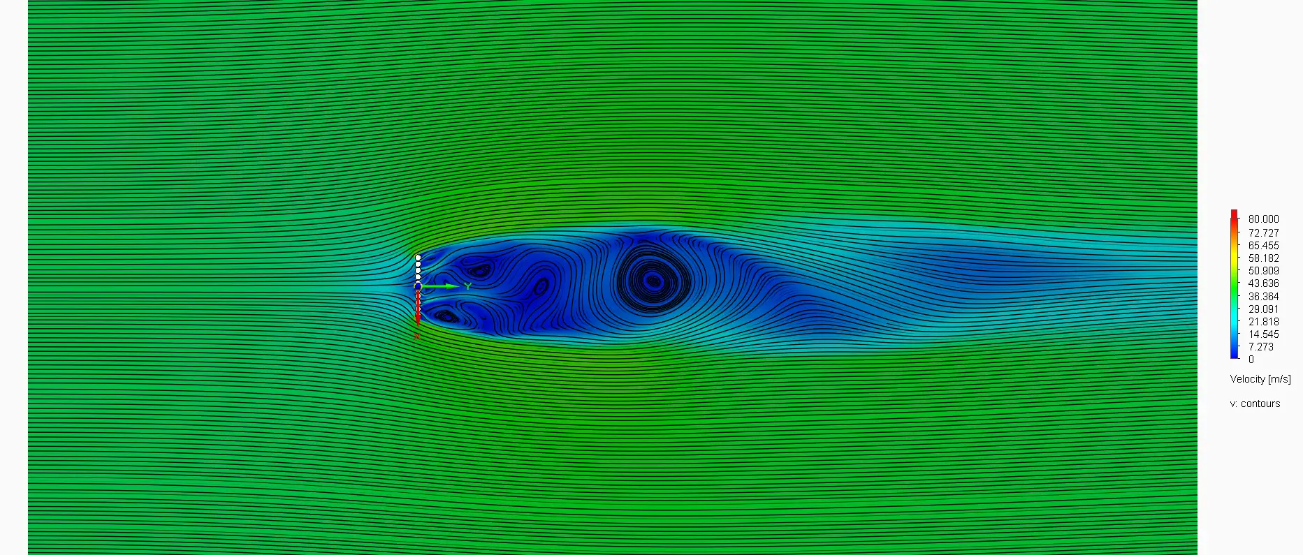
Figure 5: Example velocity field around the system for a/d ≅ 0.10
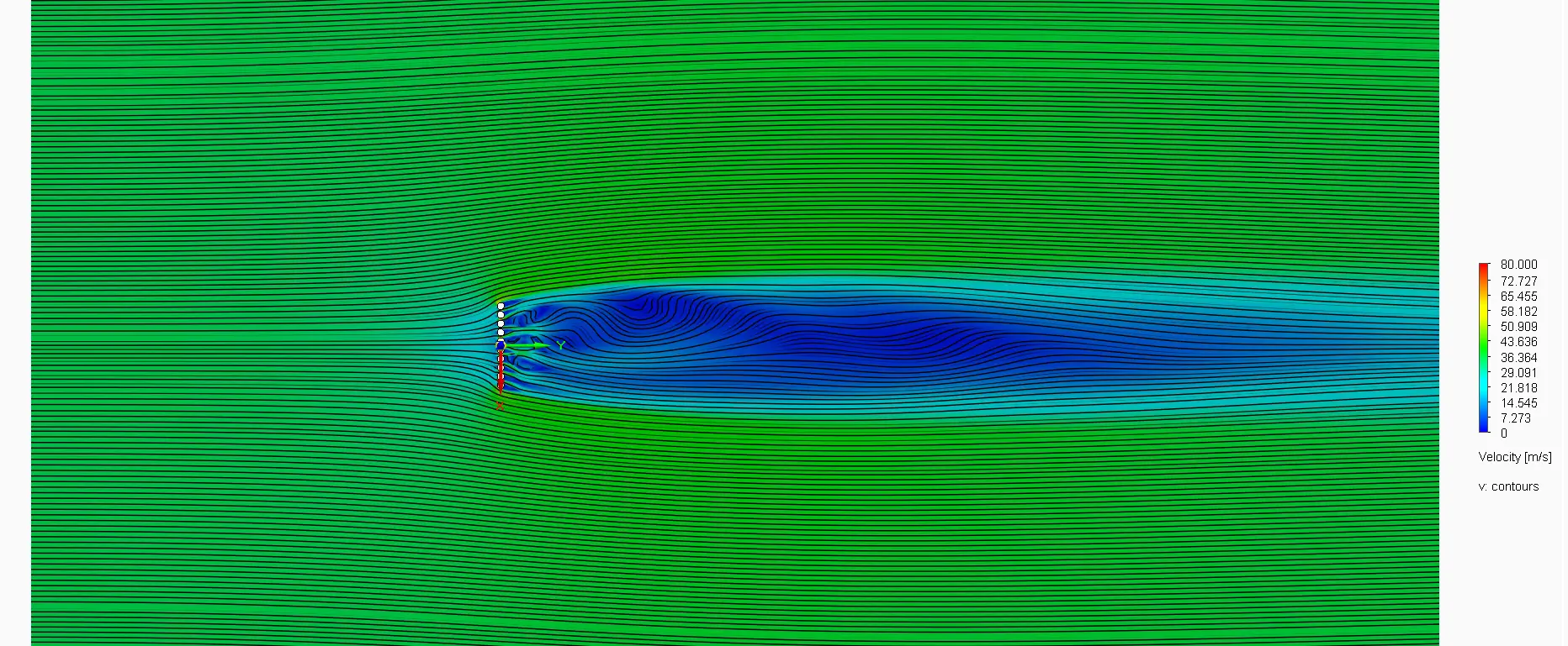
Figure 6: Example velocity field around the system for a/d ≅ 0.25
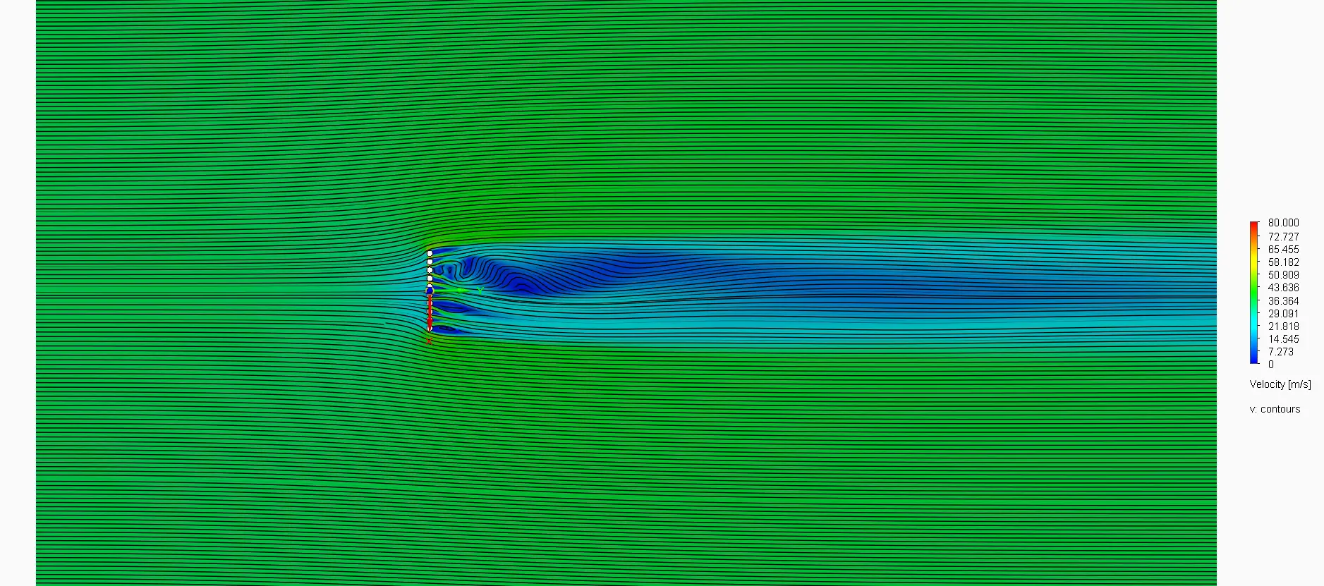
Figure 7: Example velocity field around the system for a/d ≅ 0.40
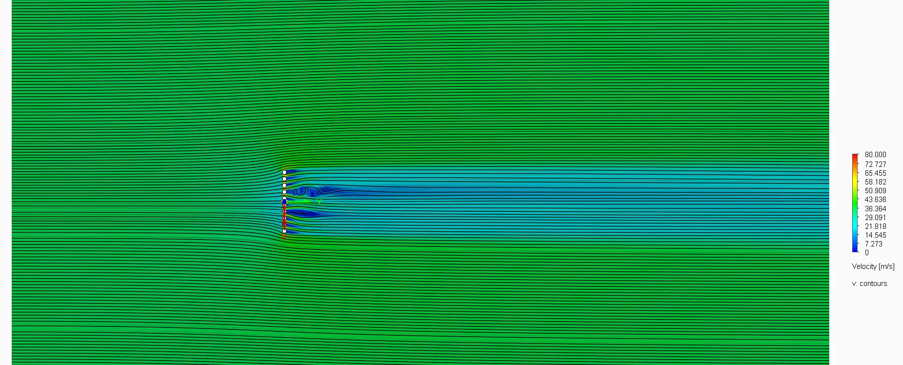
Figure 8: Example velocity field around the system for a/d ≅ 0.60
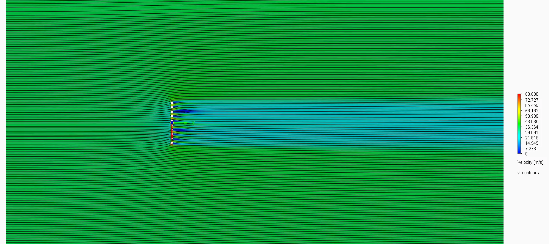
Figure 9: Example velocity field around the system for a/d ≅ 0.80
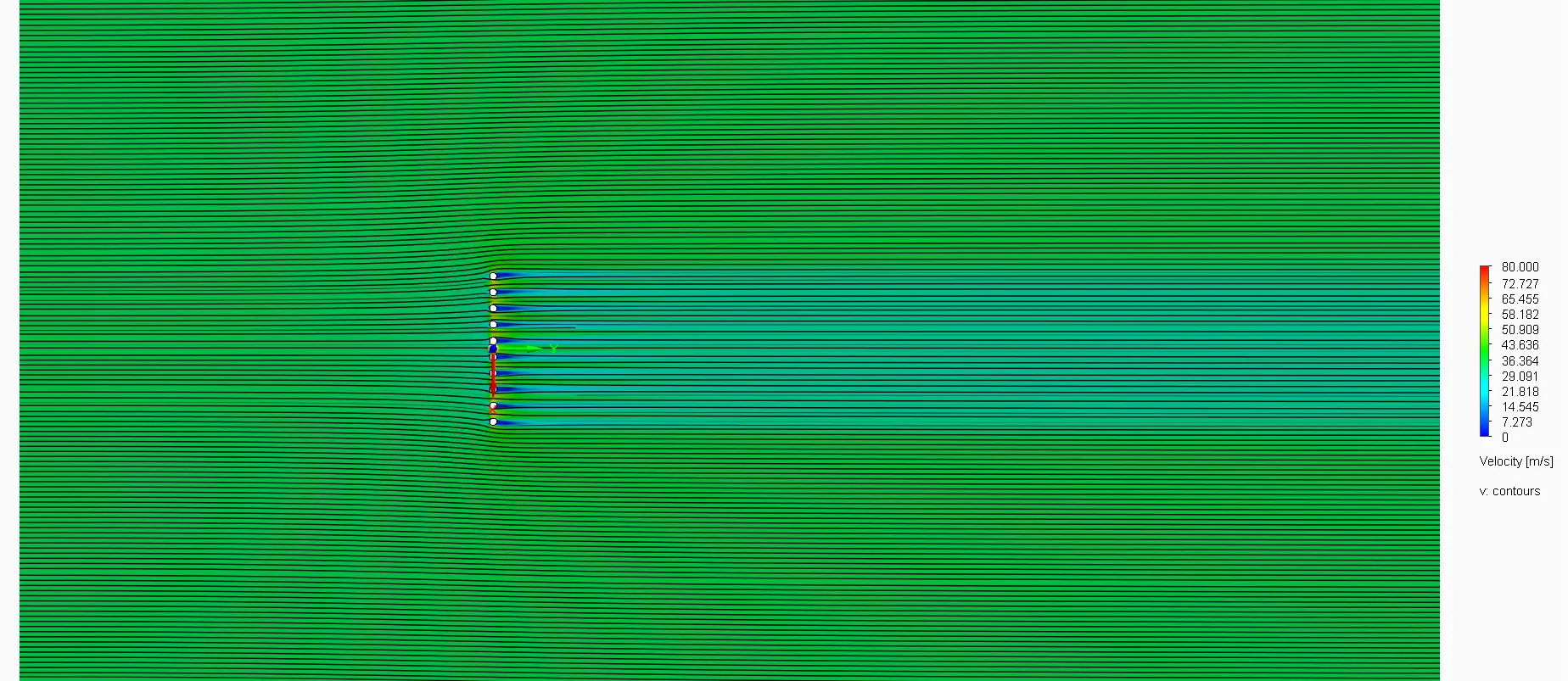
Figure 10: Example velocity field around the system for a/d ≅ 1.30
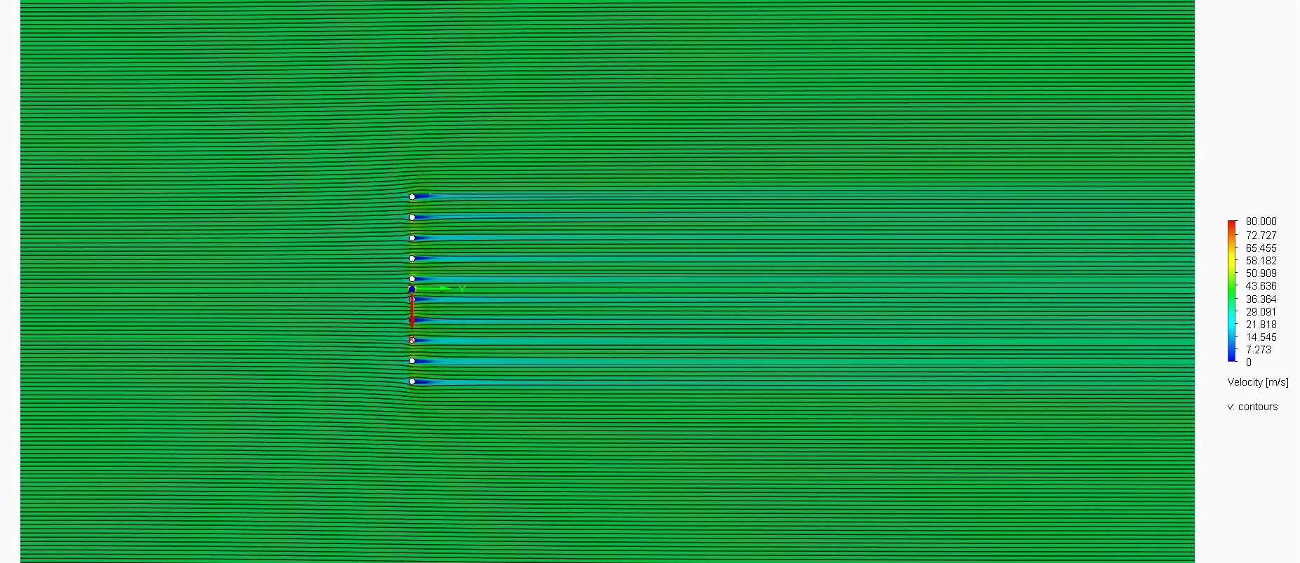
Figure 11: Example velocity field around the system for a/d ≅ 2.50
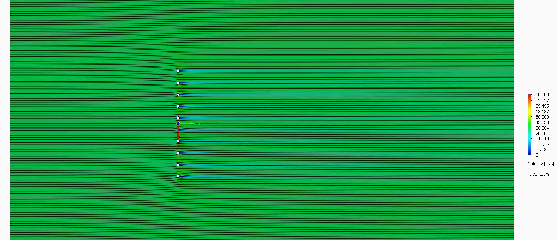
Figure 12: Example velocity field around the system for a/d ≅ 3.70
Summary
The CFD analysis examined the effect of the variable distance a (with a constant d = 15 mm) on the aerodynamic force acting on the model. The results were presented in the form of a table and a graph showing the dependence of the Cf coefficient on the a/d ratio.
The analysis revealed different characteristics of aerodynamic interactions depending on the a/d ratio, which can be divided into three ranges:
- For a/d < 1, clear aerodynamic interaction between the cables is observed, leading to elevated Cf values.
- For 1 < a/d < 3, the influence of adjacent cables is noticeable but ceases to be significant.
- Pola prędkości potwierdzają te obserwacje, pokazując zmienność rozkładu przepływu w zależności od rozstawu elementów.
- The velocity fields confirm these observations, showing the variability of the flow distribution depending on the spacing of the elements.
Concluding Remarks
The obtained CFD analysis results can be utilized in the design of wire or cable assemblies exposed to wind. For a/d values above 3, the cables can be treated as separate cylinders with independent aerodynamic behavior. However, for lower a/d values, it is necessary to apply a safety factor or conduct a detailed CFD analysis to account for the mutual interactions of the cables.
It should be noted, however, that the analysis was conducted under steady and idealized conditions, without accounting for the impact of full-scale turbulence or the effects of the cables natural vibrations, which may be significant under actual operating conditions.
